Size:
2.01
MB
EasyLife X Specification Sheet PDF
 Ce produit a été abandonné et n'est plus disponible. Vous pouvez toujours accéder à cette page à des fins d'information.


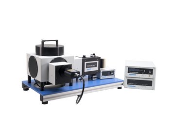
Lifetime Fluorescence Spectrometer
Though it is small and inexpensive the EasyLife™ X is a serious performer
If you have a steady state fluorometer you need a time-resolved EasyLife™ X!
The EasyLife™ X is a compact filter based fluorescence lifetime system that is an excellent companion to any lab that currently uses a steady state fluorometer but does not have access to a fluorescence lifetime system. At a fraction of the cost of a bench-top spectrofluorometer, the EasyLife™ X is extremely easy to use and yet has powerful time-resolved capabilities and decay analysis software.
Time-Resolved Fluorescence (Fluorescence Lifetimes) is an Invaluable Complement to Steady State Fluorescence (Fluorescence Spectra)
If you are currently using a steady state fluorometer for luminescence measurements, but do not have access to a fluorescence lifetime system, you should seriously consider adding the EasyLife™ X to your lab. Fluorescence intensity (steady state) and fluorescence lifetime (time-resolved) measurements are complementary. One must frequently combine results from the steady state fluorescence and the fluorescence lifetimes measurements in order to obtain the most complete information about the molecule(s) of interest. When the first modern day fluorescence lifetime instruments were introduced some thirty years ago, some investigators inherently understood the complementary nature of the fluorescence lifetime technique but it was frankly irrelevant at that time because the cost, size and complexity of those early instruments discouraged all but a relatively few from using this new time-resolved technique. Although instrumentation cost have decreased quite dramatically, as well as the size and complexity of operation, prior to the introduction of the new EasyLife™ X, it was still difficult to convince investigators to invest in a fluorescence lifetime instrument.
At a fraction of the cost of a bench-top fluorometer, and because it is just as easy to operate as a fluorometer, the introduction of the EasyLife™ X system has changed people’s attitude towards fluorescence lifetimes as a technique. Now everyone who is doing luminescence measurements can and should put fluorescence lifetimes to good use. By adding time-resolved fluorescence to your research capabilities you will finally be able to fully characterize your fluorescing molecule and molecular systems. For example, you will be able to find out what the rate constants are for the fluorescence emissions and for the non-radiative deactivation of your samples. This information is readily available by combining the lifetime results with the quantum yield values measured from the steady state instrument.
Why fluorescence lifetimes?
If you have a Steady State Fluorometer you need a Time Resolved Fluorometer to Differentiate multiple structural domains and conformations
If you want to characterize a molecule’s interactions with the surrounding environment, the steady-state measurement alone can provide a fluorescence spectrum, fluorescence quantum yield or anisotropy value, however most of this information is scrambled together, as the measured parameters are time averages and the information about specific processes is lost. This lost information becomes especially important when fluorescent molecules are used as probes to study complex systems, such as proteins, nucleic acids, quantum dots, membranes, polymers, surfactants (micelles) etc. These systems frequently exhibit multiple structural domains and conformations. The fluorescence lifetime decay curve will reveal this information by detecting multiple fluorescence lifetimes, which cannot be gleaned with a steady-state measurement where all of this information is totally obscured. The EasyLife™ X software even includes extremely powerful decay analysis software including ESM and MEM distribution analysis shown here.
Study protein conformation dynamics
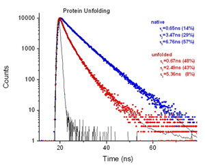
A very powerful application for a time-resolved fluorescence instrument is the study of multiple conformational states of a protein. Consider a simple case of a protein containing one Tryptophan (Trp) residue (e.g. human serum albumin HSA). With a steady state instrument all you can measure is a typical Trp spectrum reflecting no particular information about the protein, except that it contains Trp. However, if you measure the fluorescence decay, you’ll find that this single Trp residue has 4 different discrete fluorescence lifetimes! You know immediately that the protein exists in at least 4 different conformational states, and for each lifetime you know the percentage of trp residues in that state.
Quantitate binding efficiency
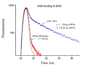
A steady state experiment can reveal binding between a fluorescent probe and a protein. Normally, the fluorescence intensity will change as a result of binding; it will either decrease or increase, depending on the nature of the probe. The information you get is very general. You detected that binding has occurred or not and that is all. However with a fluorescence lifetime system the binding will affect the probe lifetime (it will either decrease or increase for example with ANS binding to BSA), but at the same time you also detect two different lifetimes, one for the bound and the other for the unbound probe, as well as their relative contributions (pre-exponential factors) to the overall decay. From the lifetime measurement you now know relative populations of bound and unbound probes (i.e. we know the efficiency of binding).
10% Binding Efficiency
For this experiment the binding efficiency is 10% since the pre-exponential factor for the second, longer lived lifetime (the bound component) is measured as 10%. 90% of the ANS is not bound
Localize Trp in a protein
One of the major tools of fluorescence is studying quenching of fluorophores by adding quencher molecules. For example, tryptophan residues in a protein can be quenched by acrylamide or iodide ions. A steady state experiment can show the decrease of fluorescence intensity as the quencher is added, and hence that quenching has occurred, but it cannot tell you if it was dynamic or static quenching. A fluorescence lifetime experiment however will detect more than one lifetime due to different sites that Trp may occupy in the protein. Furthermore the fluorescence decay will provide the quencher effect on each lifetime, so you can get information about localization of each type of the Trp residues (e.g. are they surface exposed or buried inside the protein).
Verify you are really measuring FRET
The Förster Resonance Energy Transfer (FRET) technique has become a very powerful and wide-spread experimental tool for studying molecular binding. It is equally popular on the cellular level with fluorescence microscopes as well as in molecular solutions in cuvettes. However most investigators are using steady state techniques to observe and quantitate the ratio of fluorescence intensities of the acceptor and donor wavelengths. This has lead to a number of false conclusions and an increased awareness that the time-resolved technique is really the only way to be certain that you are actually measuring FRET.
Having a time-resolved fluorescence system is essential because the actual mechanism of fluorescence quenching in general cannot be revealed by the steady state experiment at all. There are two mechanisms that lead to quenching. The first is collisional (or dynamic) quenching, where the excited fluorophore and quencher collide and diffuse apart. The second is static quenching, where fluorophore in the ground state forms a non-fluorescent complex with quencher. In both cases the steady state experiment will show intensity decrease as more and more quencher is added. In the case of collisional (dynamic) quenching the lifetime measurement will show the lifetime decrease as more quencher is added. However, in the case of static quenching there will be no change in the lifetime at all. Discerning between the two mechanisms is critically important when one is looking to study Förster Resonance Energy Transfer (FRET). Only the time-resolved technique can prove that a ‘FRET-like’ behavior is not caused by static quenching. Only a lifetime experiment can rule it out.
Measure rotational diffusion rates and determine size of macromolecules
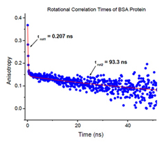
Fluorescence anisotropy (polarization) is another example of the importance of the lifetime technique. A probe molecule in a buffer will show no or very little anisotropy (ie it is not directionally dependent). Attach the probe to a protein, DNA, membrane or other large target and the fluorescence anisotropy of the probe will increase. This is all that a steady state fluorometer can tell you, that the probe is now attached to a much bigger entity. However, if you can measure the time-resolved fluorescence anisotropy of the probe, you can estimate the rate of rotational diffusion and the actual size of the macromolecule your probe is attached to. This cannot be determined with a steady state fluorometer.
Truly Affordable and Easy to Use!
The EasyLife™ X is the realization of a 40 year dream to make a small, simple, affordable fluorescence lifetime system that literally anyone can use. Using our patented fluorescence lifetime detection technique and simple snap-on pulsed LED's and laser diodes, the EasyLife™ X finally allows any researcher to be able to afford and actually conduct fluorescence lifetime experiments in their own lab.
Thinking about adding fluorescence lifetimes to your existing fluorometer?
Don't waste your money on an expensive addition to your aging fluorometer. The EasyLife™ X offers all of the same capabilities in a new, stand alone, 1 cubic foot instrument, and it will cost you less money. Plus you will have the benefit of having both your steady state fluorometer and your time resolved EasyLife™ X system both being used at the same time, dramatically increasing your labs productivity.
Skeptical that such a small, inexpensive system can do so much?
We don't blame you. It is understandable that anyone who has done fluorescence lifetime research using anything other than an EasyLife™ X could be skeptical. That is why we have compiled an extensive library of data collected on the EasyLife™ X. Please review it for samples similar to your own to see how the system could work for you. And if you don't believe us, you can also search and review literature citations using the EasyLife™.
We just can't emphasize enough how easy the EasyLife™ is to perform fluorescence lifetime experiments. There is a power button to turn on the instrument, and there is dial to adjust the stirring rate of the optional micro-stirrer for the cuvette. Everything else is controlled through the software. It is just that easy!
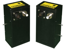
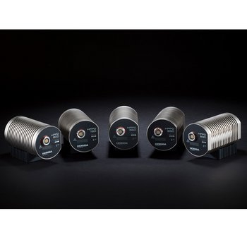
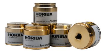
Nothing could be easier. OBB engineers have developed a broad range of simple, inexpensive, nanosecond pulsed light emitting diodes (LED's) to be used as excitation sources with the EasyLife™ systems. These small but robust light sources are available in a broad range of wavelengths, from UV to NIR. They have excellent pulse to pulse, and long term, stability in their intensity as well as their temporal pulse profiles as is evidenced by the high quality of data the system produces. Switching from one LED to another requires no alignment, and takes only a few seconds. You could not possibly work with any simpler, maintenance-free, light source for fluorescence lifetime research.
The EasyLife™ pulsed LEDs have certain distinct advantages over more conventional light sources, such as nanosecond flash lamps, lasers and laser diodes. These advantages are:
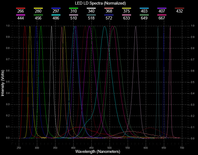
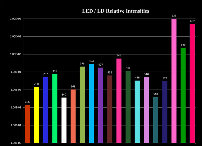
What you need to do is to select a source or sources. The following list shows you the current choices. To exchange sources is real easy, just snap off and then snap on and it is done—no alignment required.
Below 280 nm we are limited by the current state of the technology for LED’s. Do not despair the future should offer even more choic
LED Sources: | Central Wavelength | LED Sources: | Central Wavelength |
|---|---|---|---|
EL 265 | excitation LED: 266 +\- 10 nm | EL 445 | excitation LED: 444 +\- 10 nm |
EL 278 | excitation LED: 280 +\- 10 nm | EL 450 | excitation LED: 456 +\- 10 nm |
EL 295 | excitation LED: 297 +\- 10 nm | EL 490 | excitation LED: 486 +\- 10 nm |
EL 310 | excitation LED: 310 +\- 10 nm | EL 505 | excitation LED: 510 +\- 10 nm |
EL 340 | excitation LED: 340 +\- 10 nm | EL 525 | excitation LED: 518 +\- 10 nm |
EL 366 | excitation LED: 368 +\- 10 nm | EL 570 | excitation LED: 572 +\- 10 nm |
EL 375 | excitation LED: 375 +\- 10 nm | LD 630 | excitation laser diode: 633 +\- 10 nm |
EL 405 | excitation LED: 403 +\- 10 nm | LD 650 | excitation laser diode: 649 +\- 10 nm |
EL 410 | excitation LED: 407 +\- 10 nm | LD 670 | excitation laser diode: 667 +\- 10 nm |
EL 435 | excitation LED: 432 +\- 10 nm | Other LED's and laser diodes are available on request. | |
The EasyLife™ sample compartment can be configured with a variety of options including the following.
The EasyLife™ X is a time-domain fluorescence lifetime system. It collects a decay curve, allowing the user to fit the curve with comprehensive analysis software that provides many statistical tools to assess goodness of fit. The particular time-domain detection technique used in the EasyLife™ X is called the Stroboscopic technique and it is patented and unique. The Stroboscopic technique was initially developed to be a simpler, less expensive alternative to Time-Correlated Single-Photon-Counting (TCSPC). Consequently the EasyLife™ X is the world’s least expensive fluorescence lifetime system.
In addition to acquire fluorescence decays, the EasyLife™ X has the ability to measures Lifetime-Based Reaction Kinetics. If you are familiar with using a fluorometer for time-based kinetics you are familiar with collecting the steady state intensity as a function of time to monitor kinetics and reactions. The EasyLife™ X can acquire data in a similar way except that instead of the intensity changing with time the EasyLife™ X acquires, and plots in real time, the measured lifetime as a function of time. This acquisition protocol lets you measure changes in lifetimes rather than intensity. The time duration of this measurement can be from a few seconds to many hours. We believe this capability, will become an essential tool for a wide variety of emerging applications.
*If your kinetics occur on a faster timeframe then consider our new DeltaPro system that can measure lifetimes in as short a time as 1 millisecond.
The EasyLife™ X software takes full advantage of the patented stroboscopic detection hardware, to provide another unique acquisition protocol. Collecting data in a logarithmic, or arithmetic, time scale can be extremely useful for samples that have both very short and very long fluorescence lifetimes. For the short lived components you need to collect a lot of data points in order to get a good fit for those lifetimes, but for the very long lifetimes you don’t want to collect data at the same time resolution because it takes much longer and provides no benefit in fitting the decay curve.
Systems that use other techniques like TCSPC collect data in a linear time scale, so for this sample they necessarily must collect many more data points across the full acquisition time window in order to have enough data points to resolve the short lifetime components. In this way the Stroboscopic technique employed with the EasyLife™ X can easily collect excellent data for complex decay phenomena.
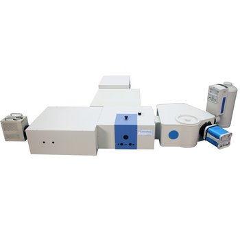
The entire EasyLife™ X takes up just one cubic foot of lab space!
With our proprietary LED light sources combined with our patented stroboscopic detection system, you are able to reap the benefits of high sensitivity, excellent temporal resolution and the unique ability to acquire lifetime kinetics or to utilize both linear and non-linear (arithmetic and logarithmic) acquisition time base. The result is a powerful and versatile lifetime instrument, capable of handling complex multi-exponential decays with an underlying broad range of lifetimes.
Did we mention that the EasyLife™ X is the easiest system available to do fluorescence lifetime experiments?
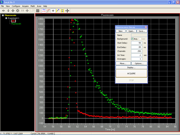
EasyLife™ software is so easy to use that literally anyone can use the system. A critical requirement to making a fluorescence lifetime system easy to use is the software, and the EasyLife™ software does the job. This is how simple the software is to use.
1. Select your Fluorescence Decay acquisition. Hit the Acquire button and within seconds or minutes depending on your settings you will have collected a decay curve. Repeat the acquisition for a scatter sample to acquire an instrument response function if necessary.
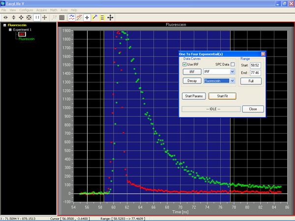
2. Analyze the decay: From the Math pull down list, select the decay model you wish to employ to fit the decay curve. Stretch the analysis window across the decay curve to determine the range for the fit. Under Start Parameters, check the number of components you want to fit. Then hit the Start Fit button. The EasyLife™ software automatically displays the resultant fitted decay curve, the measured lifetimes and a number of goodness of fit parameters such as CH1 Squared, the plot of the residuals and more. It just doesn't get any easier than that.
Don't let the price of the EasyLife™ fool you. This system comes with a totally complete set of acquisition and analysis tools for time resolved fluorescence.
In addition to acquire fluorescence decays, the EasyLife™ X has the ability to measures Lifetime-Based Reaction Kinetics. If you are familiar with using a fluorometer for time-based kinetics you are familiar with collecting the steady state intensity as a function of time to monitor kinetics and reactions. The EasyLife™ X can acquire data in a similar way except that instead of the intensity changing with time the EasyLife™ X acquires, and plots in real time, the measured lifetime as a function of time. This acquisition protocol lets you measure changes in lifetimes rather than intensity. The time duration of this measurement can be from a few seconds to many hours. We believe this capability, will become an essential tool for a wide variety of emerging applications.
*If your kinetics occur on a faster timeframe then consider our new DeltaPro system that can measure lifetimes in as short a time as 1 millisecond.
The EasyLife™ X software takes full advantage of the patented stroboscopic detection hardware, to provide another unique acquisition protocol. Collecting data in a logarithmic, or arithmetic, time scale can be extremely useful for samples that have both very short and very long fluorescence lifetimes. For the short lived components you need to collect a lot of data points in order to get a good fit for those lifetimes, but for the very long lifetimes you don’t want to collect data at the same time resolution because it takes much longer and provides no benefit in fitting the decay curve.
EasyLife™ X comes with a powerful lifetime analysis package comprising 8 different fitting programs and a FRET calculator, covering virtually all possible application scenarios. The software even includes distribution analysis for complex multi-component decay analysis. All of the fitting programs employ deconvolution as a standard option. Deconvolution removes the distortion imposed on a decay curve by a finite temporal width of the excitation pulse. It makes it possible to determine lifetimes that are 10x shorter than the excitation pulse. In order to use the deconvolution option the user must acquire an instrument response function (IRF) in addition to the fluorescence decay. The IRF can be measured by replacing the fluorescent sample with a scatterer.
Distribution analysis of multi-exponential decay
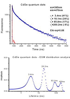
The fluorescence decay of CdSe quantum dots measured with the EasyLife™ X indicates a highly heterogeneous nature of the sample. Given that this sample had multi-exponential decays with an underlying broad range of lifetimes, the unique arithmetic progression timescale acquisition was used with this sample to greatly improve the acquisition time and analysis. This result was validated by the ESM lifetime distribution analysis tool which not only confirmed the lifetime values from the discrete 4-exponential analysis, but provides valuable information about the distribution of those discrete lifetimes
This program is suitable for the analysis of fluorescence decays consisting of up to 4 exponentials and associated pre-exponential factors. This is the most commonly used program in lifetime analysis.
The multiple file 1-to-4 exponential lifetime method allows the analysis of multiple scatterer/sample pairs as a batch operation. Each pair will be separately analyzed over the same range with the same number of exponentials and the same options. This type of analysis is useful when a series of decay curves has been collected as a function of some parameter (i.e. concentration of added reagent). Trends in the values of the lifetime parameters may then be recognized rather easily.
This program analyzes decays with up to 4 lifetimes for a number of data files simultaneously. The global analysis assumes that the lifetimes are the same among the data files but that the associated pre-exponentials are free to vary. For example, the global can be useful for analyzing various mixtures of up to 4 fluorophores.
This program is used to calculate rotational correlation times plus a residual anisotropy term. Optional polarizers are required. The program first allows the user to calculate the fluorescence lifetime(s) from the parallel and perpendicularly polarized emission intensities. The user can then calculate the rotational correlation time(s).
This program uses a “stretched exponential” fitting function (Infelta-Graetzel eqn.), which describes the quenching in micelles when added quencher molecules are Poisson distributed among the micelles. The analysis allows the determination of micellar aggregation number and the quenching rate constant.
The Maximum Entropy Method (MEM) is designed to recover lifetime distributions without any a priori assumptions about their shapes. This method uses a series of exponentials (up to 200 terms) as a probe function with fixed, logarithmically spaced lifetimes and variable pre-exponentials. This allows analyzing fluorescence decays with underlying lifetimes spanning several orders of magnitude. In many situations the MEM is capable of differentiating between continuous distributions and discrete, multi-exponentials decays. The algorithm minimizes chi-square while maximizing the entropy function at each iteration step. Ideal for complex decays, such as labeled proteins and membranes, probes adsorbed on surfaces, probes with conformational flexibility, polymers etc.
Similar to MEM, but without entropy maximization, the Exponential Series Method (ESM) is designed to recover lifetime distributions without any a priori assumptions about their shapes. This method uses a series of exponentials (up to 200 terms) as a probe function with fixed, logarithmically spaced lifetimes and variable pre-exponentials. This allows analyzing fluorescence decays with underlying lifetimes spanning several orders of magnitude. In many situations the ESM is capable of differentiating between continuous distributions and discrete, multi-exponentials decays. Ideal for complex decays, such as labeled proteins and membranes, probes adsorbed on surfaces, probes with conformational flexibility, polymers etc.
This program allows for the analysis of data by a fitting function consisting of two exponentials multiplied together and each with variable exponents of time. The exponents can be either varied or fixed which provides a powerful general function for models such as Förster energy transfer, time-dependent quenching and molecular interaction in restricted geometries (e.g. molecules on surfaces, zeolites etc.).
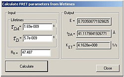
Forster Resonance Energy Transfer (FRET), sometimes referred to as Fluorescence Resonance Energy Transfer is an extremely powerful technique for the study of molecular interactions. Fluorescence lifetimes have become the technique of choice for doing FRET experiments because investigators have come to realize that FRET experiments based on steady state fluorescence measurements can sometimes result in erroneous results due to spectral shifts resulting in something other than actual FRET. The fluorescence lifetime technique lets you know if what you are looking at is really FRET. The EasyLife™ FRET Calculator calculates basic FRET parameters, such as FRET efficiency, FRET rate constant, D-A distance, and Forster radius Ro (requires spectral data from a fluorometer).
The commands in the Trace Math menu allow specific mathematical functions and operations to be carried out on individual traces or selected regions of a trace. There are 16 functions including antilog, average, distribution average, combine, xy combine, multiple derivatives, integration, linear fit, linear scaling, logarithm, normalization, reciprocal, smoothing, truncation, baseline suppression and trace merging. There is also a peak finder provided. All these functions can greatly facilitate data processing and presentation.
The EasyLife™ software that comes with the system can be loaded onto your Windows XP® laptop or computer. It loads easily on the computer and self calibrates with the instrument. Along with the QuickStart DVD you will be able to get started acquiring data right away. However, the compatibility of the EasyLife™ software with customer supplied computers is not the responsibility of OBB Corp. If you are concerned about providing your own compatible laptop or computer, we can include a laptop (with EasyLife™ software pre-loaded) on your EasyLife™ quotation so that it comes with your system. If you do decide to provide your on computer, below are the minimum specification requirements.
When we developed the EasyLife™, we knew that some people would be skeptical that an instrument that is so inexpensive, and so small and so easy to operate could possible work for them. That is why we have compiled a growing collection of data acquired on the EasyLife™. Please review the links below for samples or experiments similar to your own and see for yourself just how good the system can work for you.
Proteins
Most proteins fluoresce due to the presence of any or all three fluorescent amino acids: tryptophan, tyrosine, and phenylalanine. Intrinsic time-resolved fluorescence of tryptophan is commonly used to study the structure and dynamics of proteins. These experiments require pulsed light sources emitting in the UV, between 270 and 295 nm. The EasyLife™ X , equipped with the 280 or 295 nm pulsed LED source, is a very robust yet fast instrument perfectly suited for use with tryptophan and tyrosine fluorophores.
If you happen to use external fluorophores, there is a large selection of pulsed LEDs available for any wavelength in the UV-VIS range. A polarity sensitive, hydrophobic probe such as ANS is a good illustration of binding of an extrinsic probe to a protein.
ANS binding to bovine serum albumin was monitored with the EasyLife™ X equipped with the 370 nm LED. The lifetime of ANS in the buffer is very short, 325 ps, and increases to 8 ns upon binding to BSA. The ratio of free ANS to BSA bound ANS (9:1) can be easily determined from the double exponential fit to the fluorescence decay.
Fluorescence decays of bovine serum albumin (BSA) in PBS buffer were measured with the EasyLife™ X. The native protein shows a nearly single-exponential decay with an average lifetime of 6.31 ns. After being treated with SDS detergent, BSA undergoes a structural transition and its fluorescence decay exhibits two shorter lifetimes, 1.47 ns (37%) and 4.43 ns (63%).
If you study conformational features or hybridization of DNA, the EasyLife™ X is the right system for you. A probe molecule in a buffer will show very little or no anisotropy. Attach it to a protein, DNA, or membrane, however, and the anisotropy is increased. This is all that the steady state experiment can tell you: the probe is attached to a much bigger entity. However, if you measure the lifetime of the probe, you can estimate the rate of rotational diffusion in addition to the size of the macromolecule that is attached to the probe.
Ethidium Bromide (EB) is a commonly used DNA probe, which readily intercalates between the DNA bases. EB is weakly fluorescent in aqueous media, but becomes strongly fluorescent after intercalation into DNA. The lifetime of EB in buffer is 1.71 ns and increases dramatically to 22.7 ns after binding to calf thymus DNA.
Fluorescence decay of PicoGreen/DNA measured with an EasyLife™ X lifetime system. Conformational diversity may result in multiple lifetimes of the probe bound to DNA. The EasyLife™ X is fully capable of measuring and analyzing such complex decays. The decay of PicoGreen, a common probe for double-stranded DNA, exhibits a clearly multi-exponential behavior, resulting in three lifetimes that range from 220 ps to 9.7 ns.
The fluorescence decay of CdSe quantum dots measured with the EasyLife™ X indicates a highly heterogeneous nature of the sample. A unique feature of the EasyLife™ X, the ability to acquire data using logarithmic or arithmetic progression timescales, facilitates greatly in analysis of multi-exponential decays with an underlying broad range of lifetimes. Here, a 4-exponential decay function was needed to adequately describe the experimental decay, acquired with the arithmetic timescale. This result was validated by the ESM lifetime distribution analysis, another powerful analytical tool in the EasyLife™ X software, which confirmed the lifetime values from the discrete 4-exponential analysis.

Fluorescence decays of sample 5 in MTHF at 295 K and 77 K measured with the EasyLife™ X lifetime system equipped with the liquid nitrogen dewar attachment. The recovered lifetimes are 4.4 ns (295 K) and 7.2 ns (77 K).
Metal-ligand complexes (MLC) have become very popular probes due to their relatively long lifetimes. They are particularly suitable to studying large macromolecular systems such as nucleic acids and proteins. The figure shows a decay of one of the most common types of MLC, tris (2,2'-bipyridyl) ruthenium (II). The probe has a rather low quantum yield (about 4%). Not a problem for the EasyLife™ X! The recovered lifetime is 429 ns.
Fluorescence decay of Chl A extracted from spinach leaves and suspended in buffer. The decay is double exponential due to the presence of Chl A aggregates. The recovered lifetimes are 570 ps (93%) and 4.2 ns (7%).
Fluorescence decay of meso-tetraphenylporphyrin (m-TPP) in chloroform measured with the EasyLife™ X equipped with a 370 nm LED source. Fitted with a single exponential function, the recovered lifetime is 9.16 ns. The chi-square value of 1.07 and the random residual function indicate that the single exponential model adequately describes the decay of m-TPP.
Fluorescence decay of Rose Bengal in water measured with the EasyLife™ X lifetime system equipped with a 525-nm LED light source. Due to its highly reproducible pulse and very stable detection electronics, the EasyLife™ X is capable of measuring lifetimes, which are more than an order of magnitude shorter than the pulse width of the LED. The lifetime is determined by iterative reconvolution of the instrument response function (IRF) and the true exponential decay combined with the least squares minimization. The recovered lifetime of 94 ps is in excellent agreement with literature data citing a 92 ps lifetime for Rose Bengal in water.
One of the classical biological applications of time-resolved fluorescence spectroscopy. Typically, an elongated hydrophobic (i.e. water insoluble) molecule is used as a probe (e.g. DPH) and the anisotropy decay is measured. Due to topology of the membrane, the probe rotations are limited to the space within a cone. The rotational correlation time and the cone angle are obtained from the anisotropy data.
A very basic research area, where a fluorescing molecule is a research object on its own rather than a means of studying something else. Fluorescence lifetimes are measured in order to gain insight about the nature of electronic transition, determine radiative and nonradiative rate constants, follow excited state relaxation processes, intrinsic changes in molecular geometry, electron and energy transfer, interactions with solvent, etc.
Micelles are molecular aggregates that are formed when soaps and detergents are dissolved in water. Fluorescence decays are used mainly to determine micelle aggregation number, critical micelle concentration, polydispersity (distribution of micelle sizes) and diffusion rates in micelles.
Time resolved fluorescence is used to study intramolecular chain dynamics, end-to-end distances, secondary structure, viscosity, and association of polymers. Usual techniques are: FRET, anisotropy decays, excimer or exciplex formation and lifetimes.
Cyclodextrins (CDs) are cyclic sugar molecules that possess internal cavities capable of complexing hydrophobic organic and organometallic molecules in aqueous solution. The CDs are shaped like truncated cones with three different cavity diameters: 6.5 A (α-CD), 7.5 A (β-CD) and 9.0 A (γ-CD). Since the CDs are water soluble, but have hydrophobic interior, they can be used to deliver hydrophobic drugs. Interactions and inclusion of drugs, steroids and other molecules with the CDs have been extensively studied with the time-resolved fluorescence. The CDs are also used to study the effects of restricted geometries on the photochemistry and dynamic behavior of guest molecules.
Many molecules exhibit substantial degree of charge redistribution upon excitation. Some may even undergo a full charge separation where an electron jumps from one end of the molecule to the other. In many cases changes in molecular geometry accompany the electron transfer (e.g. TICT: twisted intramolecular charge transfer states). Such molecules are often used as fluorescent probes, since the highly polar excited states make them very sensitive to the environment. The ICT phenomenon happens also naturally, e.g. as one of primary processes in photosynthesis. Fluorescence lifetime is a common tool to study the ICT; it gives directly the rate constant for the charge transfer. Fluorescence decay kinetics, combined with time resolved fluorescence spectra could elucidate the kinetic mechanism that leads to the ICT state as well as the mechanism of subsequent relaxation.
Porphyrins and chlorophylls, compounds of great biological significance, emit fluorescence that requires NIR sensitivity. Not a problem for the EasyLife™ X, when equipped with the optional red-enhanced detector. Decays of both porphyrins and chlorophylls can be easily measured under a variety of conditions. This makes the EasyLife™ X a valuable tool for researchers studying primary processes in photosynthesis and for validation of photochemical and photophysical properties of porphyrin-based photosensitizers for photodynamic therapy.
Lifetime range | From 100 ps to 3 µs |
Dimensions | 15" x 13" x 8.8" (WxDxH) |
Weight | 25 lbs |
Sensitivity | 400 pM fluorescein or better |
Excitation | OBB proprietary pulsed nanosecond LEDs |
Optical pulse width | 1.5 ns (typical) |
Excitation range available | 280–670 nm (LED dependent) |
Emission range | 200–650 nm (optional to 900 nm) |
Emission wavelength selection | By filters |
Detection | OBB patented lifetime detector |
Typical acquisition time | 20 s (sample dependent) |
Timescale (menu selectable) | Linear, arithmetic and logarithmic |
Acquisition mode | Fluorescence Decay or Lifetime Kinetics |
Sample holder | Single 1 x 1 cm cuvette (micro-cuvettes available) |
Software | EasyLife™ X |
Lifetime analysis | Complete package: 1-to-4 exp, global, non-exponential, micelle kinetics, lifetime distribution (ESM, MEM), anisotropy, FRET calculator |
QuickStart DVD | Included |
10-nm bandpass interference filters are available individually. The peak transmittance wavelengths are 280, 289, 297, 308, 334 nm and from 340 nm to 650 nm at 10-nm increments. The filters should be used with the 507 filter holder (2 filter holders included with instrument). The bandpass filters are especially recommended for:
Set of eight 1" round longpass (cut-off) filters covering the wavelength range from 295–455 nm. Cut-off wavelengths are: 295, 305, 320, 380, 400, 420, 435 and 455 nm. The set is suitable for LED sources from 280 to 435 nm and fluorophores emitting at wavelengths above 300 nm.
Set of eight 1" round longpass (cut-off) filters covering the wavelength range from 475–610 nm. Cut-off wavelengths are: 475, 495, 515, 530, 550, 570, 590 and 610 nm. The set is suitable for LED sources from 280 to 580 nm and fluorophores emitting at wavelengths above 480 nm.
Set of eight 1" round longpass (cut-off) filters covering wavelength range from 630-1,000 nm. Cut-off wavelengths are: 630, 665, 695, 715, 780, 830, 850 and 1000 nm. The set is suitable for LED sources from 280 to 670 nm and fluorophores emitting at wavelengths above 650 nm.
Neutral density filter set. The neutral density filter set consists of six 1" round filters with approximate optical densities of 0.1, 0.3, 0.5, 1.0, 2.0 and 3.0 suitable for a spectral range of 300–2000 nm. The filters should be used with the 507 filter holder (2 filter holders included with instrument). The neutral density filters are used to decrease the signal intensity without changing the width of the emission slit. Keeping the slit constant is important for measuring decay curves and the corresponding IRF profile. For example, when a weakly fluorescent sample is measured with the widely open slit, a scatterer solution used to determine the IRF profile may saturate the PMT. A neutral density filter placed in the excitation or emission channel will bring the IRF intensity within the dynamic range of the detector without a need to change the emission slit width. This will ensure consistent illumination of the PMT photocathode and prevent potential targeting artifacts.
Polarizers are used to separate the light into vertical and horizontal components. Manual sheet polarizers are an economical solution for polarization studies that have a great acceptance angle and good throughput down to approximately 310 nm.
The 'magic angle' (MA) polarizer is a sheet polarizer with the light transmission axis oriented at 54.7 deg from the vertical. It ensures that the recorded fluorescence signal is proportional to the total emission intensity and eliminates polarization artifacts caused by emission optics. In fluorescence decay measurements it removes decay distortions caused by the rotational motion of the fluorophore. The MA polarizer should be used in the emission channel in conjunction with a vertical polarizer placed in the excitation channel.
The cold finger dewar is designed to be used with liquid nitrogen as coolant (77 K). It can also be used with organic solvent slushes at discrete temperatures above 77 K. Includes: quartz cold finger dewar that accepts 5 mm tubes, dewar holder for the single cuvette holder, foam lid for the dewar and extension collar with altered sample chamber lid, and a sample compartment. The dewar features a Suprasil quartz cold finger that passes light down to about 200 nm. Samples are placed in NMR and EPR tubes and the liquid nitrogen placed in the dewar will typically last several hours.
The front face solid sample holder insert was designed for the measurements of solid compounds or films and can be easily interchanged with the standard sample holder.
Continuously variable speed magnetic stirrer available at the time of original order. Requires a teflon-coated stirring bar (not included) suitable for a cuvette in use. Indispensable for:
The microcuvette insert supports a 3 x 3 mm 120 μl volume microcuvette with standard outer dimensions of 21 mm high by 5.4 mm wide 5.4 mm deep. The use of microcuvettes is ideal for when sample volumes are small or expensive or hard to produce such as protein work.
Vous avez des questions ou des demandes ? Utilisez ce formulaire pour contacter nos spécialistes.
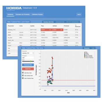
For Instant Water Quality Reports
Unlock Unprecedented Insights into Water Quality and Environmental Health
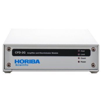
Amplifier-Discriminator
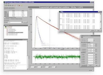
Decay Analysis Software
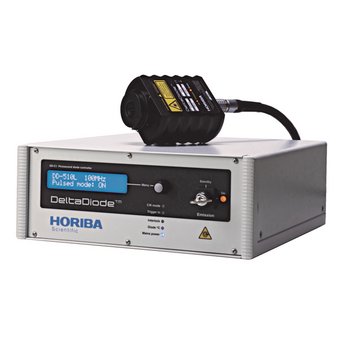
TCSPC Pulsed Sources
TCSPC/MCS Fluorescence Lifetime System
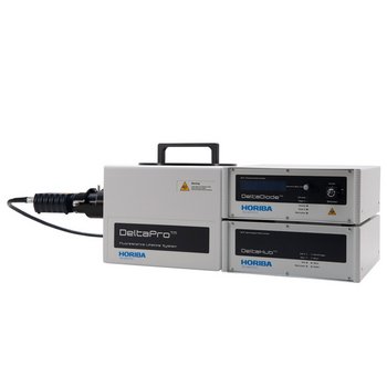
TCSPC Lifetime Fluorometer
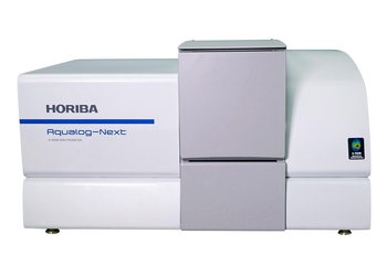
Full Spectra in Milliseconds for Industry and Academia

SPAD array imaging camera for dynamic FLIM studies at real time video rates
Modular Research Fluorometer for Lifetime and Steady State Measurements
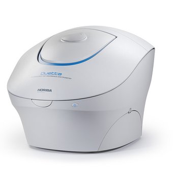
Steady State and Lifetime Benchtop Spectrofluorometer
HORIBA’s latest development in TCSPC detector technology

Spectromètre Confocal Raman à Haute Résolution

Cartographie Raman et Photoluminescence de wafers

Spectroscope Raman - Microscope d'imagerie automatisé
Système Raman Polyvalent
Steady State and Lifetime Nanotechnology EEM Spectrofluorometer

For Single‐Walled Carbon Nanotube Excitation‐Emission Map Simulation and Analysis
Single photons detection with picosecond accuracy
PLQY Integrating Sphere
LED Phosphorescence Light Sources
Spectromètre Raman abordable à ultra-basse fréquence, jusqu'à 10 cm-1
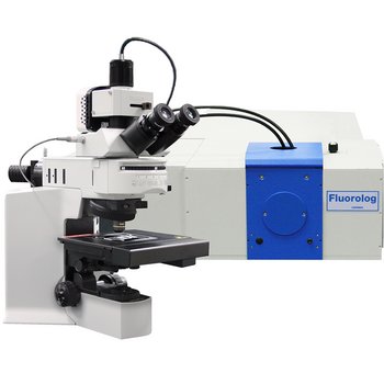
Connect any of our steady state and hybrid fluorometers to virtually any upright or inverted microscope!
Spectromètre Micro-Raman - Microscope Raman Confocal